Advanced Formulas in MS Excel
Lesson Goals
- Learn about naming and labeling cells and ranges of cells.
- Learn to use names and labels in formulas.
- Learn to create formulas that span multiple worksheets.
- Learn to use the conditional
IFfunction and its variants in formulas. - Learn to use the
PMTfunction to calculate payments for loans. - Learn to use the
LOOKUPfunction. - Learn to use the
VLOOKUPfunction. - Learn to use the
HLOOKUPfunction. - Learn to use the
CONCATfunction to join the contents of numerous cells. - Learn to use the
TRANSPOSEfunction. - Learn to use the
PROPER,UPPER, andLOWERfunctions to alter the casing of text. - Learn to use the
LEFT,RIGHT, andMIDfunctions to return characters from the start or end of a string, or a specific number of text characters. - Learn to use various date functions.
Using Named Ranges in Formulas
Some of the advantages to naming and labeling cells include:
- Using names can make it easier to understand what a formula does (e.g.,
=Q3Sales*Commission). - Names work throughout a workbook, so using names can simplify the process of creating formulas that span multiple sheets.
Here is a list of things you need to know about cell names:
- The first character of a name must be either a letter, a backslash (\), or an underscore (_).
- Other (non-first) characters can be letters, numbers, underscores, or periods.
- Spaces cannot be used.
- The maximum number of characters in a name is 255.
- Anything that could be a cell reference (e.g., C10, $B$7) cannot be used as a name.
- Names are not case sensitive (e.g., the names "total", "Total", and "TOTAL" are the same in Excel).
Naming a Single Cell
To name a cell:
- Select the cell you wish to name.
- In the Name Box (to the left of the formula bar), type the name:

- Press Enter.
Naming a Range of Cells
To name a range of cells:
- Select the cells in the range you wish to name.
- In the Name Box (to the left of the formula bar), type the name:

- Press Enter.
Naming Multiple Single Cells Quickly
To quickly name cells using their row and column headings:
- Select the rows and columns containing the range you wish to name:

- On the Formulas tab, in the Defined Names group, click the Create from Selection command:

- In the Create Names from Selection dialog box, check the desired boxes and click OK:

- In the following image, cells can now be referred to using the row and column headings:

Hint: If step 3 isn't working for you, make sure that you named cell B1 "QuarterlyIncome" with no space and that you did not include a space within "QuarterlyIncome" in the formula for B13.
Using Named Ranges in Formulas
Duration: 10 to 20 minutes.
In this exercise, you will practice naming cells and will use named cells in a formula.
- Open Using Names.xlsx from your Excel2019.2/Exercises folder.
- Name cell B1 "Quarterly Income".
- Use the Create from Selection command to name cells in the range A3:E8.
- Using only names in your formulas, answer the questions in column A of the worksheet.
Solution:
- To name cell B1:
- Select cell B1.
- Type "QuarterlyIncome" in the Name Box and press Enter:
 .
.
- To name cells A3:E8:
- Select cells A3:E8.
- On the Formulas tab, in the Defined Names group, click the Create from Selection command:

- In the Create Names from Selection dialog box, check Top row and Left column and click OK:

- To answer the questions in column A of the worksheet:
- How much was spent on Clothes and Fun Stuff in January? Type "
=Jan Clothes+Jan Fun_Stuff". - How much was spent on Groceries in Jan and Mar? Type "
=Jan Groceries+Mar Groceries". - What % of Quarterly Income did Electric account for from Jan to Mar? Type "
=Total Electric/QuarterlyIncome".
- How much was spent on Clothes and Fun Stuff in January? Type "
Using Formulas That Span Multiple Worksheets
To create a formula that spans multiple worksheets:
- If you haven't named cells, then:
- Select the sheet and cell into which you wish to type the formula.
- Type "
=". - Select the sheet that includes the data you will use in your formula.
- Select the cell that contains the data.
- Enter an operator (
+,-,*,/). - Either select another cell in that sheet or select another sheet and cell to complete the formula.
- If your formula contains named cells or ranges, simply:
- Select the sheet and cell into which you wish to type the formula.
- Type "
=". - Enter the formula using names.
Entering a Formula Using Data in Multiple Worksheets
Duration: 10 to 20 minutes.
In this exercise, you will enter a formula using data from multiple sheets first without names and then using named cells.
- Open Multiple Worksheets.xlsx from your Excel2019.2/Exercises folder.
- Answer the questions in rows 3, 4, and 5 of Sheet2 using the data in Sheet1 without using named cells.
- Answer the questions in rows 10, 11, and 12 of Sheet2 using the data in Sheet1 using named cells. Note: The cells are already named.
Solution:
- To answer the questions in rows 3, 4, and 5:
- How much was spent on Clothes and Fun Stuff in January?
- Type "
=". - Select Sheet1 by clicking on it.
- Select cell B7.
- Type "
+". - Select cell B8.
- Press Enter.
- The formula you entered will read: "
=Sheet1!B7+Sheet1!B8".
- Type "
- How much was spent on Groceries in Jan and Mar?
- Type "
=". - Select Sheet1 by clicking on it.
- Select cell B4.
- Type "
+". - Select cell D4.
- Press Enter.
- The formula you entered will read: "
=Sheet1!B4+Sheet1!D4".
- Type "
- What percent of Quarterly Income did Electric account for from Jan to Mar?
- Type "
=". - Select Sheet1 by clicking on it.
- Select cell E5.
- Type "
/". - Select cell B1.
- Press Enter.
- The formula you entered will read: "
=Sheet1!E5/QuarterlyIncome".
- Type "
- How much was spent on Clothes and Fun Stuff in January?
- To answer the questions in rows 10, 11, and 12:
- How much was spent on Clothes and Fun Stuff in January? Type "
=Jan Clothes+Jan Fun_Stuff". - How much was spent on Groceries in Jan and Mar? Type "
=Jan Groceries+Mar Groceries". - What percent of Quarterly Income did Electric account for from Jan to Mar? Type "
=Total Electric/QuarterlyIncome".
- How much was spent on Clothes and Fun Stuff in January? Type "
Using the IF Function
The
IF function can be used to execute formulas only under certain conditions or to execute different formulas based on specified conditions. This is known as conditional logic. To use the IF function, you need to know:- Logical Test. This is simply the thing you want to test. For example:
- If the number is greater than 10, then...
- If the value is "blue", then...
- Value if True. This is the value to return if the requirement is met (the logical test is true).
- Value if False. This is the value to return if the requirement is not met (the logical test is false).
Here are some things to know about the
IF function:- In plain English, the
IFfunction says: If X condition is true, put Y value in this cell; otherwise, put Z value in the cell. - The value returned by the
IFfunction can be a number, text, a formula, or a reference to another cell. - Enter "" (open and close quotes) if you do not wish to return a value.
- You can test up to seven conditions by nesting
IFfunctions within the originalIFfunction. Here is an example in which nestedIFfunctions are used to return grades:
To use the
IF function:- On the Formulas tab, in the Function Library group, click the Insert Function command:

- In the Insert Function dialog box:
- Search on "IF" or, in the Or select a category drop-down box, select Logical.
- Under Select a function, select IF.
- Click OK.

- In the Function Arguments dialog box:
- Enter the logical test (e.g.,
B2>10,B2<C2,B2="Blue"). - Type in the value if true.
- Type in the value if false.
- Click OK.

- Enter the logical test (e.g.,
Using AND/OR Functions
The
AND and OR functions are similar to the IF function in that they are logical functions.
The syntax of the AND function is:
=AND(logical1,logical2, ...). It returns TRUE if all arguments are true.
The syntax of the OR function is:
=OR(logical1,logical2, ...). It returns TRUE if any arguments are true.
Note that when you see a small picture of a worksheet with a red arrow on it next to a data entry field, you can click this image to select a cell, rather than typing the cell's location into the data entry field. For example:
- Click the circled image:

- The Function Arguments dialog box opens up. Click a cell and the cell's location appears in the Function Arguments dialog box. Click the image to the far right of the Function Arguments dialog box to return to the previous dialog box:

- Note that in the original dialog box, the selected cell's location has been added into the data entry field:

This is especially useful when referring to cells on a separate worksheet.
Here are some examples of the
IF statement in use:=IF(A1=B1,"Same","Different"):
=IF(A1="Blue",B1,C1):
- =
IF(A1>100,"Victory!","Try again."):
Using the SUMIF, AVERAGEIF, and COUNTIF Functions
SUMIF
There are a few variations of the IF function that may be useful to be aware of when working with Excel.
The
SUMIF function is a variation of the IF function, which allows you to specify criteria for a sum. For example, you may want to sum only the numbers in a column that are above 100.
To use
SUMIF, you need to know:- range. The range of cells to which you want to apply the criteria.
- criteria. This can be text, numbers, a function, or an expression. For example, the criteria could be > 100.
AVERAGEIF
AVERAGEIF does what it sounds like: it averages a range of cells. For example, you could average students' grades in a spreadsheet.
To use
AVERAGEIF, you need to know:- range. Enter a range of at least two cells to which to apply the criteria.
- criteria. The criteria defines what is to be averaged, such as numbers, expressions, and text.
COUNTIF
The
COUNTIF function allows you to count the number of cells in a range that meet the criteria you specify. For example, you can count the number of students who received As.
To use the COUNTIF function, you need to know:
- range. Enter a range of at least two cells to which to apply the criteria.
- criteria. The criteria defines what is to be averaged, such as numbers, expressions, and text.
Using the IF Function
Duration: 15 to 25 minutes.
In this exercise, you will practice using the
IF function.- Open Functions.xlsx from your Excel2019.2/Exercises folder and go to the sheet named "IF".
- Use the
IFfunction to enter "Yes" or "No" in column E based on whether revenue from each customer exceeded $10,000 (i.e., if revenue exceeded $10,000, enter "Yes"; otherwise, enter "No"). - Use the
IFfunction to enter "Yes" or "No" in column F based on whether the number of purchases from each customer was greater than or equal to 20 (i.e., if # of purchases exceeded 19, enter "Yes"; otherwise, enter "No".) - Use the
IFfunction to enter the revenue received from customers located in Utica, and only Utica, in column G (i.e., if the customer is located in Utica, enter revenue; otherwise, leave blank).
Solution:
- Use the
IFfunction to enter "Yes" or "No" in column E based on whether revenue from each customer exceeded $10,000.- The information you need to enter this formula is:
- Logical Test: If revenue is greater than $10,000, then...
- Value if True: "Yes"
- Value if False: "No"
- The formula is:
=IF(B2>10000,"Yes","No") - Enter the formula using the Insert Function command:
- Select cell E2.
- On the Formulas tab, in the Function Library group, click the Insert Function command:

- In the Insert Function dialog box:
- Search on "IF" or, in the Or select a category drop-down box, select Logical.
- Under Select a function, select IF.
- Click OK.

- In the Function Arguments dialog box, enter the following values and click OK:
- Logical_test: B2>10000
- Value_if_true: "Yes"
- Value_if_false: "No"

- Copy the formula from cell E2 to cells E3:E8.
- The information you need to enter this formula is:
- Use the
IFfunction to enter "Yes" or "No" in column F based on whether the number of purchases from each customer was greater than or equal to 20.- The information you need to enter this formula is:
- Logical Test: If the number of purchases is greater than 19, then...
- Value if True: "Yes"
- Value if False: "No"
- The formula is:
=IF(C2>19,"Yes","No") - Enter the formula using the Insert Function command:
- Select cell F2.
- On the Formulas tab, in the Function Library group, click the Insert Function command:
- In the Insert Function dialog box:
- Search on "IF" or, in the Or select a category drop-down box, select Logical.
- Under Select a function, select IF.
- Click OK.
- In the Function Arguments dialog box, enter the following values and click OK:
- Logical_test: C2>19
- Value_if_true: "Yes"
- Value_if_false: "No"

- Copy the formula from cell F2 to cells F3:F8.
- The information you need to enter this formula is:
- Use the
IFfunction to enter the revenue received from customers located in Utica, and only Utica, in column G.- The information you need to enter this formula is:
- Logical Test: If city is Utica, then...
- Value if True: Revenue (B2)
- Value if False: None ("")
- The formula is:
=IF(D2="Utica",B2,"") - Enter the formula using the Insert Function command:
- Select cell G2.
- On the Formulas tab, in the Function Library group, click the Insert Function command:
- In the Insert Function dialog box:
- Search on "IF" or, in the Or select a category drop-down box, select Logical.
- Under Select a function, select IF.
- Click OK.
- In the Function Arguments dialog box, enter the following values and click OK:
- Logical_test: D2="Utica"
- Value_if_true: B2
- Value_if_false: ""

- Copy the formula from cell G2 to cells G3:G8.
- The information you need to enter this formula is:
Using the PMT Function
The
PMT function is used to calculate payments on loans. In order to use the PMT function, you need to know:- Rate. The interest rate.
- Nper. The number of payments.
- Pv. The present value of the future payments, or the amount of the loan.
- Fv. The future value, or the cash balance after the final payment has been made. NOTE: the cash balance is not the remaining balance of the loan. Instead, it is the cash on hand after the loan is paid off. If the loan won't be completely paid off, then the future value is a negative number.
- Type. Whether the payments are made at the beginning or end of each period.
To use the
PMT function:- On the Formulas tab, in the Function Library group, click the Insert Function command:

- In the Insert Function dialog box:
- Search on "Payment" or, in the Or select a category drop-down box, select Financial.
- Under Select a function, select PMT.
- Click OK.

- In the Function Arguments dialog box:
- Enter the interest rate (Rate) or the cell in which it is located. If your worksheet contains the annual interest rate and payments will be made monthly, then select the annual rate and divide by 12.
- Enter the number of payments (Nper).
- Enter the present value (Pv).
- Enter the future value (Fv). If you leave this blank, Excel will assume the future value is $0.
- For Type, enter "0" if payments are made at the end of the period and "1" if payments are made at the beginning of the period. If you leave this blank, Excel will assume payments are made at the end of the period.
- Click OK.

Here are some examples:
- To calculate a 24-month $3,000 loan with 9% interest, assuming the loan is to be completely paid off and payments are made at the end of each period:
=PMT(0.09/12,24,3000,0,0)or=PMT(0.09/12,24,3000):
- To calculate a 15-year $200,000 loan with 6% interest, assuming half the loan is to be paid off and payments are made at the end of each period:
=PMT(0.06/12,180,200000,-100000): Note that 15 years = 180 months.
- To calculate a 15-year $200,000 loan with 6% interest, assuming half the loan is to be paid off and payments are made at the beginning of each period:
=PMT(0.06/12,180,200000,-100000,1):
Using the PMT Function
Duration: 15 to 25 minutes.
In this exercise, you will...
- Open Functions.xlsx from your Excel2019.2/Exercises folder and go to the sheet named "PMT".
- Calculate the payments for Loans 1, 2, 3, and 4.
- Assume you purchased a house for $240,000 and took out a 30-year mortgage for the whole amount with an interest rate of 6%. What is your payment? Enter the formula in cell B9.
- Assume you purchased a car for $29,000 and took out a loan for the whole amount with an interest rate of 9%. You are to pay off $20,000 of the loan in 4 years. Payments are to be made at the beginning of each period. What is your payment? Enter the formula in cell B10.
Solution:
- Loan 1:
- Formula: "
=PMT(C2/12,D2,B2,E2)" - Solution:
- On the Formulas tab, in the Function Library group, click the Insert Function command:

- In the Insert Function dialog box, select PMT and click OK:

- In the Function Arguments dialog box, enter the following values and click OK:
- Rate: C2/12
- Nper: D2
- Pv: B2
- Fv: E2
- Type: Leave blank.

- On the Formulas tab, in the Function Library group, click the Insert Function command:
- Formula: "
- Loan 2:
- Formula: "
=PMT(C3/12,D3,B3)" - Solution:
- On the Formulas tab, in the Function Library group, click the Insert Function command.
- In the Insert Function dialog box, select PMT and click OK.
- In the Function Arguments dialog box, enter the following values and click OK:
- Rate: C3/12
- Nper: D3
- Pv: B3
- Fv: Leave blank.
- Type: Leave blank.

- Formula: "
- Loan 3:
- Formula: "
=PMT(C4/12,D4,B4)" - Solution:
- On the Formulas tab, in the Function Library group, click the Insert Function command.
- In the Insert Function dialog box, select PMT and click OK.
- In the Function Arguments dialog box, enter the following values and click OK:
- Rate: C4/12
- Nper: D4
- Pv: B4
- Fv: Leave blank.
- Type: Leave blank.

- Formula: "
- Loan 4:
- Formula: "
=PMT(C5/12,D5,B5,E5,1)" - Solution:
- On the Formulas tab, in the Function Library group, click the Insert Function command.
- In the Insert Function dialog box, select PMT and click OK.
- In the Function Arguments dialog box, enter the following values and click OK:
- Rate: C5/12
- Nper: D5
- Pv: B5
- Fv: E5
- Type: 1.

- Formula: "
- Assume you purchased a house for $240,000 and took out a 30-year mortgage for the whole amount with an interest rate of 6%. What is your payment?
- The formula is:
=PMT(0.06/12,360,240000) - To solve this using the Insert Function command:
- On the Formulas tab, in the Function Library group, click the Insert Function command.
- In the Insert Function dialog box, select PMT and click OK.
- In the Function Arguments dialog box, enter the following values and click OK:
- Rate: 0.06/12
- Nper: 360
- Pv: 240000
- Fv: Leave blank.
- Type: Leave blank.

- The formula is:
- Assume you purchased a car for $29,000 and took out a loan for the whole amount with an interest rate of 9%. You are to pay off $20,000 of the loan in 4 years. Payments are to be made at the beginning of each period. What is your payment?
- Formula:
=PMT(0.09/12,48,29000,9000,1) - To solve this using the Insert Function command:
- On the Formulas tab, in the Function Library group, click the Insert Function command.
- In the Insert Function dialog box, select PMT and click OK.
- In the Function Arguments dialog box, enter the following values and click OK:
- Rate: 0.09/12
- Nper: 48
- Pv: 29000
- Fv: 9000
- Type: 1.

- Formula:
Using the LOOKUP Function
The LOOKUP function returns a value either from a one-row or one-column range or from an array. The LOOKUP function has two syntax forms: the vector form and the array form.
To use the
LOOKUP function, you need to know:- Lookup value. The value you will use to identify individual records in your table.
- Lookup vector. For a vector syntax, this will be a range that contains one row or column.
- Array. For an array syntax, this is the range you want to compare with the lookup value.
To use the
LOOKUP function:- On the Formulas tab, in the Function Library group, click the Insert Function command:

- In the Insert Function dialog box:
- Search on "LOOKUP" or, in the Or select a category drop-down box, select Lookup & Reference.
- Under Select a function, select LOOKUP.
- Click OK.

- In the Select Arguments dialog box, choose a vector or array syntax and click OK.

- In the Function Arguments dialog box (the following is for a vector):
- Enter the Lookup_value.
- Enter the Lookup_vector.
- Enter the Result_vector.
- Click OK.

Using the VLOOKUP Function
The
VLOOKUP function is used to pull a value from a list or table based on a corresponding value. For example, if you have a worksheet with a table showing employee names, hire date, and salary, you could use VLOOKUP in a separate worksheet to pull the hire date and salary for individual employees from the first worksheet. In this example, the employee name serves as a key, identifying which information from the first worksheet you wish to pull.
To use the
VLOOKUP function, you need to know:- Lookup value. The value you will use to identify individual records in your table. The Lookup Value must be in the left-most column of your table.
- Table array. The table that contains the data you will use
VLOOKUPto retrieve. This table can be in another worksheet or even another workbook from the one in which you enter theVLOOKUPfunction. - Col index num. The Lookup Value is always in the left-most column of the Table Array (column #1, regardless of where in the worksheet the table is located). The next column to the right is column #2, then column #3, etc. The Col index num is simply the number of the column that contains the value you wish to retrieve.
- Range lookup. Enter False if the Lookup Value must match exactly. If you enter True or leave blank, Excel will assume the table is sorted in ascending order and will select the best match. Note that if the table is not sorted in ascending order, Excel likely won't correctly find the best match.
To use the
VLOOKUP function:- On the Formulas tab, in the Function Library group, click the Insert Function command:

- In the Insert Function dialog box:
- Search on "VLOOKUP" or, in the Or select a category drop-down box, select Lookup & Reference.
- Under Select a function, select VLOOKUP.
- Click OK.

- In the Function Arguments dialog box:
- Enter the Lookup_value or the cell in which it is located.
- Enter the Table_array.
- Enter the Col_index_num.
- Enter the Range_lookup. If you leave this blank, Excel will treat this as if you entered True.
- Click OK.

Using the VLOOKUP Function
Duration: 15 to 25 minutes.
In this exercise, you will use the
VLOOKUP function to automatically fill in the description and price of items on an invoice based on the item number.- Open VLOOKUP.xlsx from your Excel2019.2/Exercises folder and go to the sheet named "Invoice".
- Use the
VLOOKUPfunction to query the Description and Price from the table located in the sheet named "Table". You will need to insert theVLOOKUPfunction into cells B7:B15 and D7:D15.- Hint: Including absolute references when referring to the range will enable the formulas to be copied to other cells within the column.
- What is Item Number 135798 and what does it cost?
- What is Item Number 678452 and what does it cost?
Solution:
- To query the Description from the table located in the sheet named "Table":
- In the sheet named "Invoice", select cell B7.
- On the Formulas tab, in the Function Library group, click the Insert Function command:

- In the Insert Function dialog box:
- Search on "VLOOKUP" or, in the Or select a category drop-down box, select Lookup & Reference.
- Under Select a function, select VLOOKUP.
- Click OK.

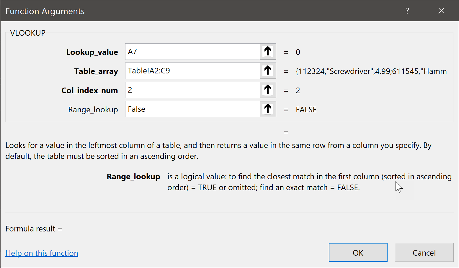
- In the Function Arguments dialog box:
- Enter the Lookup_value: A7.
- Enter the Table_array: Table!A2:C9 (click the cell selection arrow, then the sheet named "Table", and then select the cells).
- Enter the Col_index_num: 2 (because the description is in the second column in the table).
- Enter the Range_lookup: False (because you require an exact match).
- Click OK.
- To query the Price from the table located in the sheet named "Table":
- In the sheet named "Invoice", select cell D7.
- On the FORMULAS tab, in the Function Library group, click the Insert Function command.
- In the Insert Function dialog box:
- Search on "VLOOKUP" or, in the Or select a category drop-down box, select Lookup & Reference.
- Under Select a function, select VLOOKUP.
- Click OK.
- In the Function Arguments dialog box:
- Enter the Lookup_value: A7.
- Enter the Table_array: Table!A2:C9 (click the cell selection arrow, then the sheet named "Table", and then select the cells).
- Enter the Col_index_num: 3 (because the description is in the third column in the table).
- Enter the Range_lookup: False (because you require an exact match).
- Click OK.
- Select cell B7 and edit the formula to make the table references absolute (change A2:C9 to $A$2:$C$9). Then do the same in cell D7.
- Copy cell B7 to cells B8:B15 and cell D7 to D8:D15.
- Enter "135798" into any cell under "Item Number" on the invoice. Item Number 135798 is a rake and costs $12.98.
- Enter "678452" into any cell under "Item Number" on the invoice. Item Number 678452 is a wrench and costs $6.99.
Using the HLOOKUP Function
The
HLOOKUP function is very similar to the VLOOKUP function. The only significant difference is that while the VLOOKUP function looks for a value in the left-most column of a table and returns a value on the same row as that value, the HLOOKUP function looks for a value in the top row of a table and returns a value in the same column as that value. To use the HLOOKUP function, you need to know:- Lookup value. The value you will use to identify individual records in your table. The Lookup Value must be in the top row of your table.
- Table array. The table that contains the data you will use
HLOOKUPto retrieve. This table can be in another worksheet or even another workbook from the one in which you enter theHLOOKUPfunction. - Row index num. The Lookup Value is always in the top row of the Table Array (row #1, regardless of where in the worksheet the table is located). The next row down is row #2, then row #3, etc. The Row index num is simply the number of the row that contains the value you wish to retrieve.
- Range lookup. Enter False if the Lookup Value must match exactly. If you enter True or leave blank, Excel will assume the table is sorted in ascending order and will select the best match. Note that if the table is not sorted in ascending order, Excel likely won't correctly find the best match.
To use the
HLOOKUP function:- On the Formulas tab, in the Function Library group, click the Insert Function command:

- In the Insert Function dialog box:
- Search on "HLOOKUP" or, in the Or select a category drop-down box, select Lookup & Reference.
- Under Select a function, select HLOOKUP.
- Click OK.

- In the Function Arguments dialog box:
- Enter the Lookup_value or the cell in which it is located.
- Enter the Table_array.
- Enter the Row_index_num.
- Enter the Range_lookup. If you leave this blank, Excel will treat this as if you entered True.
- Click OK.

Using the CONCAT Function
The
CONCAT function (called CONCATENATE in versions of Excel previous to 2019) is used to join the contents of multiple cells. For example, if you have a worksheet with first names in one column and last names in another column, you can use the CONCAT function to join the first and last names into one column. This function supports cell references, as well as range references.
Here are some things to know about the
CONCAT function:- You can join up to 255 text strings.
- The text string can include text, numbers, and cell references.
- You can include text not found in the worksheet by adding it via the Function Arguments dialog box (or directly into the formula). For example, if you have a worksheet with city names in one column and state names in another column, and wish to join them into one column, you can add a comma and space (", ") between the two.
To use the
CONCAT function:- On the Formulas tab, in the Function Library group, click the Insert Function command:

- In the Insert Function dialog box:
- Search on "CONCAT" or, in the Or select a category drop-down box, select Text.
- Under Select a function, select CONCAT.
- Click OK.

- In the Function Arguments dialog box:
- In the Text1 data entry field, enter the first text field or the cell in which it is located.
- In the Text2 data entry field, enter the first text field or the cell in which it is located.
- Etc. (New fields appear when you use the bottom field.)
- Click OK.

Using the CONCAT Function
Duration: 10 to 15 minutes.
In this exercise, you will practice using the
CONCAT function.- Open Functions.xlsx from your Excel2019.2/Exercises folder and go to the sheet named "CONCATENATE".
- Use the
CONCATfunction to join the first and last names into full names in column C. - Use the
CONCATfunction to join the cities and states so that they appear as "city, state".
Solution:
- To join the first and last names into full names:
- In the sheet named "CONCAT", select cell C2.
- On the Formulas tab, in the Function Library group, click the Insert Function command:

- In the Insert Function dialog box:
- Search on "CONCAT" or, in the Or select a category drop-down box, select Text.
- Under Select a function, select CONCAT.
- Click OK.

- In the Function Arguments dialog box:
- In the Text1 data entry field, enter cell A2.
- In the Text2 data entry field, enter a space (" ").
- In the Text3 data entry field, enter cell B2.
- Click OK.

- Copy cell C2 to cells C3:C7.
- To join the cities and states so that they appear as "city, state":
- In the sheet named "CONCAT", select cell G2.
- On the Formulas tab, in the Function Library group, click the Insert Function command.
- In the Insert Function dialog box:
- Search on "CONCAT" or, in the Or select a category drop-down box, select Text.
- Under Select a function, select CONCAT.
- Click OK.
- In the Function Arguments dialog box:
- In the Text1 data entry field, enter cell E2.
- In the Text2 data entry field, enter a comma and a space (", ").
- In the Text3 data entry field, enter cell F2.
- Click OK.

- Copy cell G2 to cells G3:G7.
Using the TRANSPOSE Function
You can use the
TRANSPOSE function to return a horizontal range of cells as a vertical range or a vertical range as a horizontal range.
To use
TRANSPOSE, you must know the array, the range of cells you want to transpose. To use the TRANSPOSE function:- On the Formulas tab, in the Function Library group, click the Insert Function command:

- In the Insert Function dialog box:
- Search on "TRANSPOSE" or, in the Or select a category drop-down box, select Recommended.
- Under Select a function, select TRANSPOSE.
- Click OK.

- In the Function Arguments dialog box:
- In the Array data entry field, enter the range of cells or an array of values you want to transpose.
- Click OK.

Using the PROPER, UPPER, and LOWER Functions
The
PROPER function is used to make the first letter in each word uppercase and all other letters lowercase. To use the PROPER function:- On the Formulas tab, in the Function Library group, click the Insert Function command:

- In the Insert Function dialog box:
- Search on "PROPER" or, in the Or select a category drop-down box, select Text.
- Under Select a function, select PROPER.
- Click OK.

- In the Function Arguments dialog box:
- In the Text data entry field, enter the cell containing the text you wish to capitalize the first letters of.
- Click OK.

The UPPER Function
The
UPPER function is used to make all letters in words uppercase.- On the Formulas tab, in the Function Library group, click the Insert Function command:
- In the Insert Function dialog box:
- Search on "UPPER" or, in the Or select a category drop-down box, select Text.
- Under Select a function, select UPPER.
- Click OK.

- In the Function Arguments dialog box:
- In the Text data entry field, enter the cell containing the text you wish to make all uppercase.
- Click OK.

The LOWER function
The
LOWER function is used to make all letters in words lowercase.- On the Formulas tab, in the Function Library group, click the Insert Function command:
- In the Insert Function dialog box:
- Search on "LOWER" or, in the Or select a category drop-down box, select Text.
- Under Select a function, select LOWER.
- Click OK.

- In the Function Arguments dialog box:
- In the Text data entry field, enter the cell containing the text you wish to make all lowercase.
- Click OK.

The TRIM Function
Another text function you may use is the TRIM function.
TRIM allows you to remove the spaces in phrases, leaving only single spaces between words.The LEN Function
Another text function that may be useful is the LEN function.
LEN allows you to determine a text string's length.Using the PROPER Function
Duration: 5 to 10 minutes.
In this exercise, you will practice using the
PROPER function.- Open Functions.xlsx from your Excel2019.2/Exercises folder and go to the sheet named "PROPER".
- In column B, use the
PROPERfunction to capitalize the first letters of the names in column A.
Solution:
- To capitalize the first letters of the names in column A:
- In the sheet named "PROPER", select cell B2.
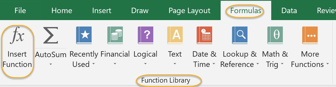
- On the Formulas tab, in the Function Library group, click the Insert Function command:

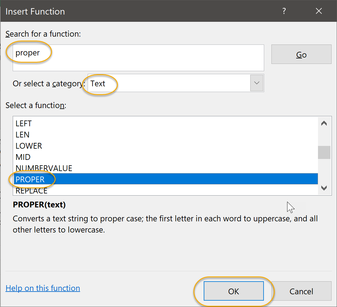
- In the Insert Function dialog box:
- Search on "PROPER" or, in the Or select a category drop-down box, select Text.
- Under Select a function, select PROPER.
- Click OK.
- In the Function Arguments dialog box:
- In the Text data entry field, enter A2.
- Click OK.

- Copy cell B2 to cells B3:B7.
Using the LEFT, RIGHT, and MID Functions
The
LEFT and RIGHT functions are used to return characters from the start or end of a string. For example, you could use the LEFT and RIGHT functions to:- Return the area codes from a list of phone numbers (if the phone numbers are formatted as 315-333-4444, you would use the
LEFTfunction to return the first three characters). - Return the zip codes from a list of addresses (if the addresses are formatted as Syracuse, NY 13210, you would use the
RIGHTfunction to return the last five characters). - Return a piece of an identifying ID (if you have a list of IDs in which the first four digits represent a product, the next six digits represent the date, and the last three digits represent the store the product was sold from, you could use the
LEFTfunction to return the four digits representing the product or theRIGHTfunction to return the three digits representing the store the product was sold from).
To use the
LEFT and RIGHT functions:- On the Formulas tab, in the Function Library group, click the Insert Function command:

- In the Insert Function dialog box:
- Search on "LEFT" or "RIGHT" or, in the Or select a category drop-down box, select Text.
- Under Select a function, select LEFT or RIGHT.
- Click OK.

- In the Function Arguments dialog box:
- In the Text field, enter the cell containing the text string from which you wish to return characters.
- In the Num_Chars field, enter the number of characters you want to return.
- Click OK.

The MID Function
The
MID function is used when you want to return a specific amount of characters from a string of text. You specify the number of characters.
To use the MID function:
- On the Formulas tab, in the Function Library group, click the Insert Function command:
- In the Insert Function dialog box:
- Search on "MID" or, in the Or select a category drop-down box, select Text.
- Under Select a function, select MID.
- Click OK.

- In the Function Arguments dialog box:
- In the Text field, enter the text characters that you wish to return.
- In the Start_num field, enter the position of the first character that you wish to extract.
- In the Num_Chars field, enter the number of characters you want to return.
- Click OK.

Excel 2016 inroduced a number of new functions, including the following. To view all of the functions, click each button in the Function Library.
DECIMALfunction: Available on the Math & Trig tab. This function converts the text of a number in a given base into a decimal number.ACOTfunction: Available on the Math & Trig tab. This function returns the arccotangent of a number.ENCODEURLfunction: Available on the More Functions tab in the Web section. This function returns a URL-encoded string.DAYSfunction: Available on the Date & Time tab. This function shows the number of days between two dates.
Excel 2019 then added some more new functions:
IFS: Tests conditions in the order you specify.MINIFS: Returns the smallest function in a range (which meets the criteria).MAXIFS: Returns the largest function in a range (which meets the criteria).SWITCH: Used to return the first matching result of the evaluation of an expression against a list of values in order.TEXTJOIN: Used to combine text from different ranges; each item is separated by a delimiter.
Using the LEFT and RIGHT Functions
Duration: 5 to 15 minutes.
In this exercise, you will practice using the
LEFT and RIGHT functions.- Open Functions.xlsx from your Excel2019.2/Exercises folder and go to the sheet named "LEFT-RIGHT".
- In column B, use the
LEFTfunction to display only the area codes of the phone numbers listed in column A. - In columns E and F, use the
LEFTandRIGHTfunctions to display the Store IDs and Salesperson IDs for the sales listed in column D.
Solution:
- To display only the area codes of the phone numbers listed in column A:
- In the sheet named "LEFT-RIGHT", select cell B2.
- On the Formulas tab, in the Function Library group, click the Insert Function command:

- In the Insert Function dialog box:
- Search on "LEFT" or, in the Or select a category drop-down box, select Text.
- Under Select a function, select LEFT.
- Click OK.

- In the Function Arguments dialog box:
- In the Text field, enter cell A2.
- In the Num_Chars field, enter the number "3".
- Click OK.

- Copy cell B2 to cells B3:B7.
- To display the Store IDs for the sales listed in column D:
- In the sheet named "LEFT-RIGHT", select cell E2.
- On the Formulas tab, in the Function Library group, click the Insert Function command.
- In the Insert Function dialog box:
- Search on "LEFT" or, in the Or select a category drop-down box, select Text.
- Under Select a function, select LEFT.
- Click OK.
- In the Function Arguments dialog box:
- In the Text field, enter cell D2.
- In the Num_Chars field, enter the number "3".
- Click OK.

- Copy cell E2 to cells E3:E7.
- To display the Salesperson IDs for the sales listed in column D:
- In the sheet named "LEFT-RIGHT", select cell F2.
- On the Formulas tab, in the Function Library group, click the Insert Function command.
- In the Insert Function dialog box:
- Search on "RIGHT" or, in the Or select a category drop-down box, select Text.
- Under Select a function, select RIGHT.
- Click OK.

- In the Function Arguments dialog box:
- In the Text field, enter cell D2.
- In the Num_Chars field, enter the number "2".
- Click OK.

- Copy cell F2 to cells F3:F7.
Using Date Functions
The three most commonly used date functions are
YEAR, MONTH, and DAY. These functions are used to return only the year, month, or day from a date. To use the YEAR, MONTH, and DAY functions:- On the Formulas tab, in the Function Library group, click the Insert Function command:

- In the Insert Function dialog box:
- Search on "Year", "Month", or "Day" or, in the Or select a category drop-down box, select Date & Time.
- Under Select a function, select YEAR, MONTH, or DAY.
- Click OK.

- In the Function Arguments dialog box:
- In the Serial_number field, enter the cell in which the full date is located.
- Click OK.

Using the NOW and TODAY Functions
Two other date functions are
NOW and TODAY. They are useful when you need to show the current date information or need to calculate something based on that information.NOW: Returns the current date and time.TODAY: Returns the current date, but the time is set to 12:00:00 AM.
Using the YEAR, MONTH, and DAY Functions
Duration: 5 to 15 minutes.
In this exercise, you will practice using the
YEAR, MONTH, and DAY functions.- Open Functions.xlsx from your Excel2019.2/Exercises folder and go to the sheet named "Date".
- Use the
YEAR,MONTH, andDAYfunctions to add the years, months, and days of the dates found in column A to columns B, C, and D.
Solution:
- To add the year of the dates found in column A to column B:
- In the sheet named "Date", select cell B2.
- On the Formulas tab, in the Function Library group, click the Insert Function command:
- In the Insert Function dialog box:
- Search on "Year" or, in the Or select a category drop-down box, select Date & Time.
- Under Select a function, select YEAR.
- Click OK.

- In the Function Arguments dialog box:
- In the Serial_number field, enter cell A2.
- Click OK.

- Copy cell B2 to cells B3:B6.
- To add the month of the dates found in column A to column C:
- In the sheet named "Date", select cell C2.
- On the Formulas tab, in the Function Library group, click the Insert Function command:
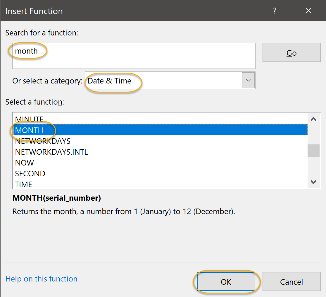
- In the Insert Function dialog box:
- Search on "Month" or, in the Or select a category drop-down box, select Date & Time.
- Under Select a function, select MONTH.
- Click OK.
- In the Function Arguments dialog box:
- In the Serial_number field, enter cell A2.
- Click OK.

- Copy cell C2 to cells C3:C6.
- To add the day of the dates found in column A to column D:
- In the sheet named "Date", select cell D2.
- On the Formulas tab, in the Function Library group, click the Insert Function command:
- In the Insert Function dialog box:
- Search on "Day" or, in the Or select a category drop-down box, select Date & Time.
- Under Select a function, select DAY.
- Click OK.

- In the Function Arguments dialog box:
- In the Serial_number field, enter cell A2.
- Click OK.

- Copy cell D2 to cells D3:D6.
Creating Scenarios
In Excel 2013 and later, scenarios are input values that you can create and save, which return different calculated results. You can use them in what-if scenarios.
Utilize the Watch Window
The Watch Window is a feature that allows you to keep formulas that you need to view in sight, rather than having to jump around in a worksheet.
To use the Watch Window:
- Select the Formulas tab, and in the Formula Auditing group, select Watch Window.

- In the worksheet, select the cells you want to watch and click Add Watch in the Watch Window.

- In the Add Watch dialog box, click Add.

Consolidate Data
To consolidate data from multiple worksheets into one master worksheet:
- Select the Data tab, and from the Data Tools tab, select Consolidate.

- While in the Consolidate dialog box, click and drag to select cells.
- Use the Add button to continue to add data, and click OK when you are done.

Enable Iterative Calculations
You can enable iterative calculations to locate circular references.
To enable iterative calculations:
- From the File menu tab, select Options.
- Select the Formulas section, and from the Calculation options section, check the Enable iterative calculation check box.

What-If Analyses
The Data tab's Forecast group (in Excel 2013, the Data Tools group) contains the What-If Analysis drop-down list, which contains a number of what-if tools. One of these tools is Goal Seek.
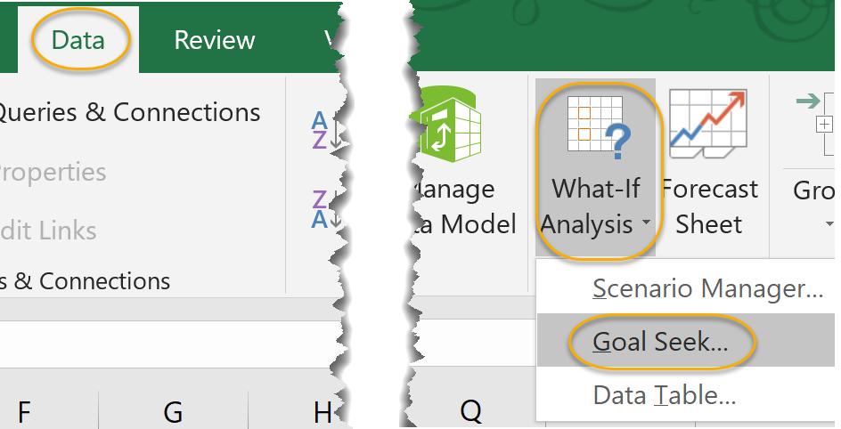
To use Goal Seek:
- Select the cell with the formula you are going to solve for.
- Select the Data tab, and in the Forecast group (Data Tools group in Excel 2013), select What-If Analysis, and then select Goal Seek.

- In the To value field, enter the goal.

- In the By changing cell field, enter the cell where you want the result to be and then click OK.

Use the Scenario Manager
To manage what-if models so you can quickly access them, you can use the Scenario Manager.
To use the Scenario Manager:
- Select the Data tab, and in the Forecast group (Data Tools group in Excel 2013), select What-If Analysis, and then select Scenario Manager.

- In the Scenario Manager dialog box, click Add. Type a name for the scenario in the Scenario name text box, and in the Changing cells text box, type the names of the cells you want to change and click OK.

- In the Scenario Values dialog box that appears, type the values for the changing cells.

- Click Add to add more scenarios and click OK when you are done.
Use Financial Functions
The Excel financial functions are complex financial formulas that contain multiple steps. These functions cover things as calculating net present value, the depreciation of an asset, and loan payments, amongst others.
To access the financial functions, from the Formulas tab, in the Function Library group, select Financial. 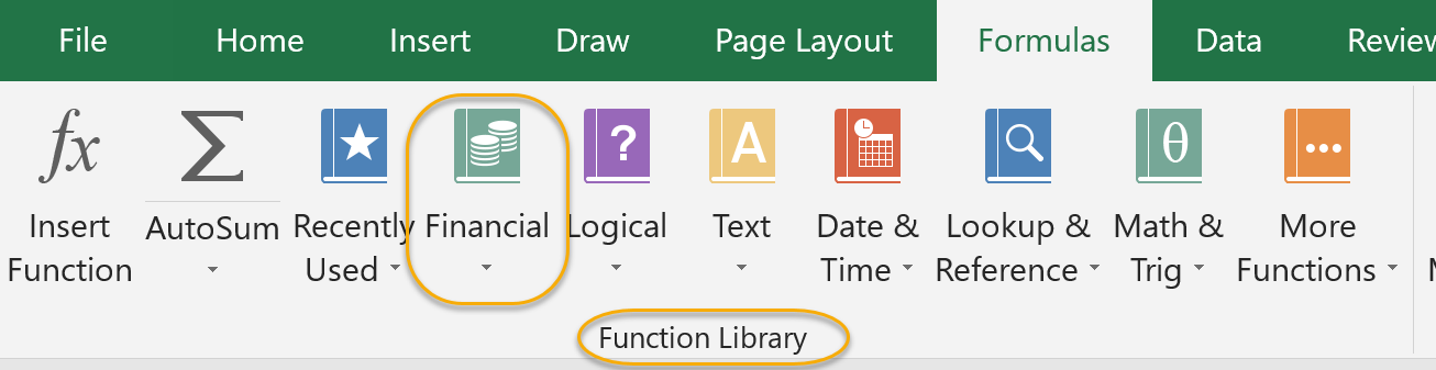


Comments
Post a Comment